REINFORCEMENT LEARNING

Last updated on: May 26, 2024

Definition of reinforcement learning

• Concerned with the foundational issue of learning to make good (optimality in context) sequences of decisions.
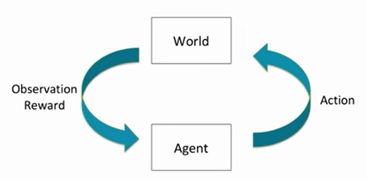
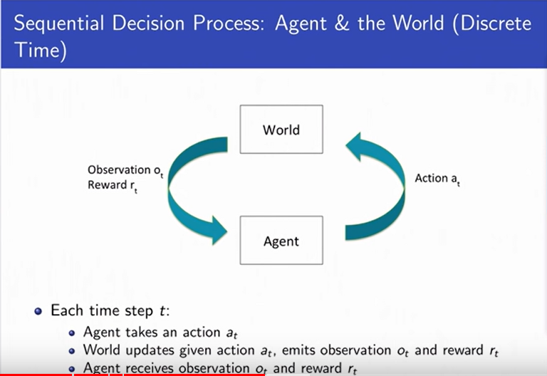
• Intelligent systems need to make decision. Learning agents are required to perform actions based on the environment.
• An example of this is playing video game based on pixel inputs, take nececcary actions to get reward.
• Application in robotics- optimize

Key aspects of reinforcement learning

1. Optimization
• Goal to find an optimal way to make decisions
• Yielding best outcomes
• Or at least a very good strategy
2. Delayed consequences
• Decisions now can impact things much later (results not known) such as saving for retirement or finding a key in Montezuma's revenge
• Introduces two challenges:
  1. When planning: decisions involve reasoning about not just immediate benefit but also its longer term ramifications
  2. When learning: temporal credit assignment is hard (what caused later high or low rewards?)
3. Exploration

How do we explore?

• Learning about the world by making decisions
  1. Agent as scientist
  2. Learn to ride a bike by tyring (and failing)
  3. Finding a key in Montezuma's revenge- Traveler's diarrhea (dysentery, Montezuma's revenge) is usually a self-limiting episode of diarrhea that results from eating food or water that is contaminated with bacteria or viruses. Traveler's diarrhea is most common in developing countries that lack resources to ensure proper waste disposal and water treatment.
• A challange here is Censored data
  1. Only get a reward (label) for decision made
  2. Don't know what would have happened if we had taken red pill instead of blue pill.
• Decision impact what we learn about- If we choose college A or B, we will have different later experiences.
4. Generalization

What is decision policies? Mapping from experiences to decision and why this need to be learned?

• Policy is mapping from past experience to action.
• Why not just pre-program a policy? - Why not write everythin as a program as a series of IF-THEN-ELSE statement? Answer- As it will be absolutely enormous and not tractable.

AI Planning (vs RL)

• Optimization
• Generalization
• Exploration
• Delayed consequences
• Computes good sequence of decisions
• But given a model of how decisions impact world

Supervised Machine Learning (vs RL)

• Optimization
• Generalization
• Exploration
• Delayed consequences
• Learn from experience
• But provided correct labels

Unsupervised Machine Learning (vs RL)

• Optimization
• Generalization
• Exploration
• Delayed consequences
• Learn from experience
• But no labels from world

Imitation Learning

Imitation Learning, also known as Learning from Demonstration (LfD), is a method of machine learning where the learning agent aims to mimic human behavior. In traditional machine learning approaches, an agent learns from trial and error within an environment, guided by a reward function. However, in imitation learning, the agent learns from a dataset of demonstrations by an expert, typically a human. The goal is to replicate the expert's behavior in similar, if not the same, situations.
Imitation learning represents a powerful paradigm in machine learning, enabling agents to learn complex behaviors without the need for explicit reward functions. Its application spans numerous domains, offering the potential to automate tasks that have traditionally required human intuition and expertise. As research in this field continues to advance, we can expect imitation learning to play an increasingly significant role in the development of intelligent systems.

• Reduces RL to supervised learning
• Benefits
  • Great tools for supervised learning
  • Avoids exploration problem
  • With big data lots of data about outcomes of decisions
• Limitations
  • Can be expensive to capture
  • Limited by data collected
• Imitation learning + RL promising!

Imitation Learning vs RL

• Optimization
• Generalization
• Exploration
• Delayed consequences
• Learn from experience...of others
• Assumes input demos of good policies

How to proceed with RL?

• Explore the world
• Use experience to guide future decisions

Issues with RL

• Where do rewards come from? And what happens if we get it wrong?
• Robustness / Risk sensitivity
• Multi-agent RL

Sequential Decision Making Under Uncertainity

	Goal: Select actions to minimize total expected future reward. May require balancing immediate & long term rewards May require strategic behaviour to achieve high rewards. The world can also be an agent. Example: Web advertisement, Robot unloading dishwasher, blood pressure control

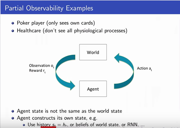
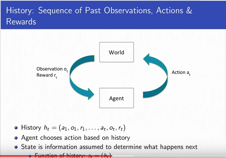
Markov Assumption

• It says that the state used by an agent is a sufficient statistic of history.
• In order to predict the future, you only need the current state of the environment.
• Future is independent of the past given present.

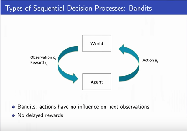
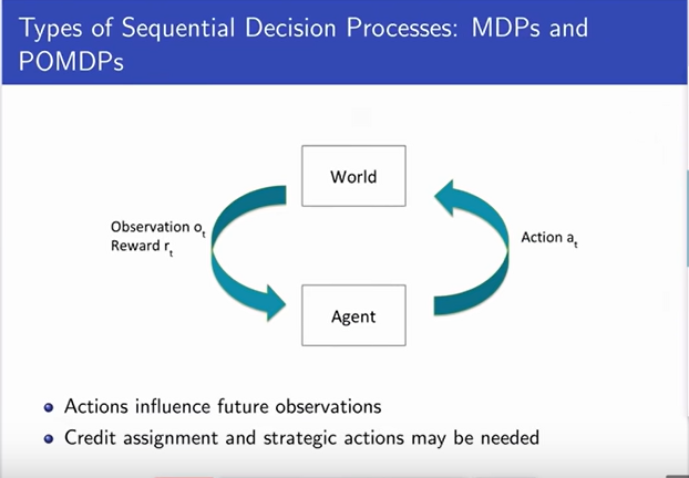
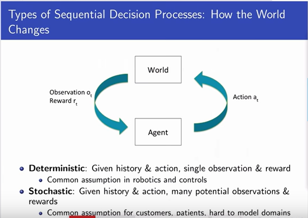
Types of Sequential Decision Making Process

RL Algorithm Components

Often include one or more of
• Model: Representation of how the world changes in response to agent's action.
  • Agent's representation of how the world changes in response to agent's action
  • Transition / dynamics model predicts next agent state
  • Reward model predicts immediate reward

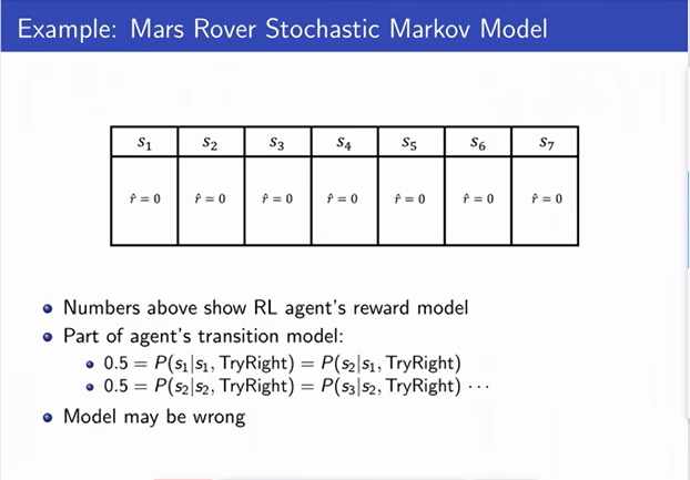
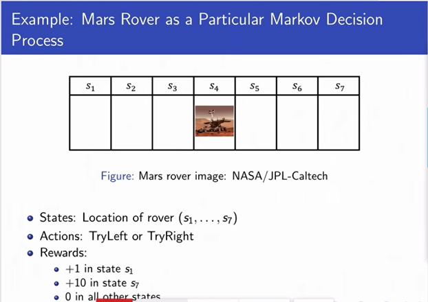
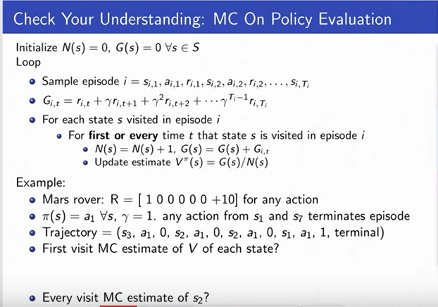
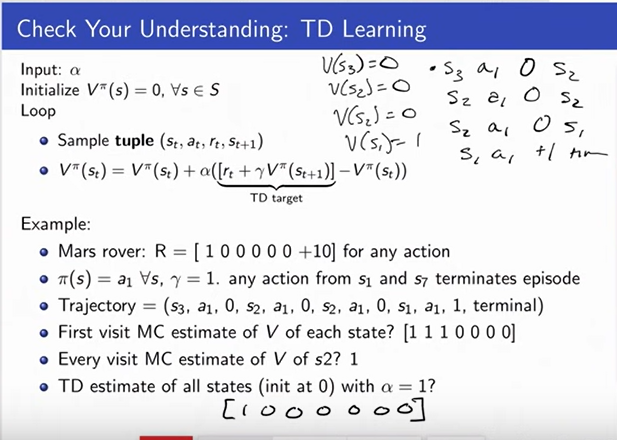
  Lets say, rotor control is very bad and there is 50% probability the the rover moves and 50% that it does not move. 0 reward everywhere. Model can be wrong. As the actual reward is 1 in state s1 and 10 in state s7

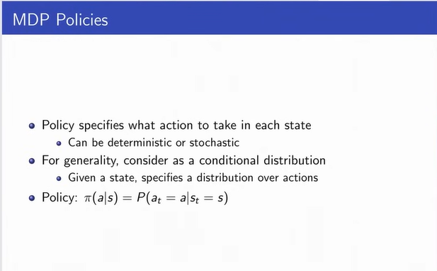
• Policy: Function mapping agent's states to actions
  • Policy or decision policy is simply how we make decisions.
  • Mapping from states to actions.
  • Deterministic policy means there is only one action.
  • Stochastic policy means you can have a distribution over actions you might take.
• Value function: Future rewards from being in a state and/or action when following a particular policy.
  • Value function is expected discounted sum of future rewards under a particular policy.
  • Its a weighting which says how much reward do I get now and in the future. Weighted by how much I care about immediate vs long term rewards.
  • The Discount factor y (gamma) weighs immediate vs future rewards. It is between 0 and 1.
  • Value function allows us to say how good or bad the different states are.
  • Can be used to quantify goodness/badness of states and actions
  • And decide how to act by comparing policies.

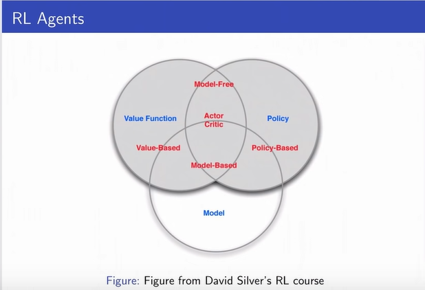
Types of RL Agents

• Model-based
  • Explicit: Model
  • May or may not have policy and/or value function
• Model-free
  • Explicit: Value function and/or policy function
  • No model

RL Agents

Key Challanges in Learning to Make Sequences of Good Decicions

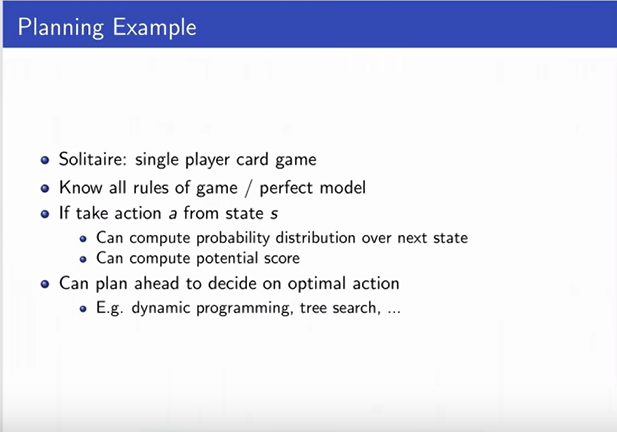
Planning Example

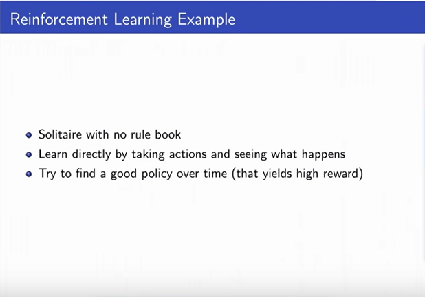
Reinforcement Learning Example

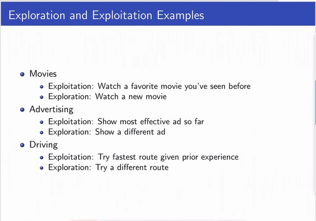
Exploration and Exploitation

• Agent only experiences what happens for the actions it tries
• Mars rover trying to drive left learns the reward and next state for trying to drive left, but not for trying to drive right
• Obvious! But leads to a dilema - Things which are good based on the prior experience and things which will be good in future.
• How should RL agent balance its actions?
• Exploration: trying new things that might enable the agent to make better decisions in the future.
• Exploitation: choosing actions that are expected to yield good reward given past experience.
• Often there may be an exploration-exploitation tradeoff
• May have to sacrifice reward in order to explore & learn about potentially better policy

Exploration and Exploitation Examples

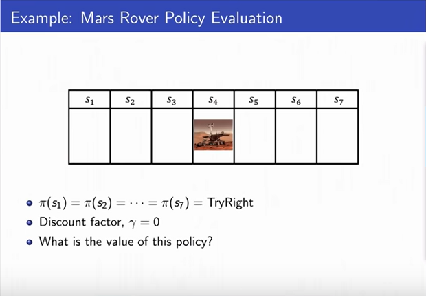
Evaluation and Control

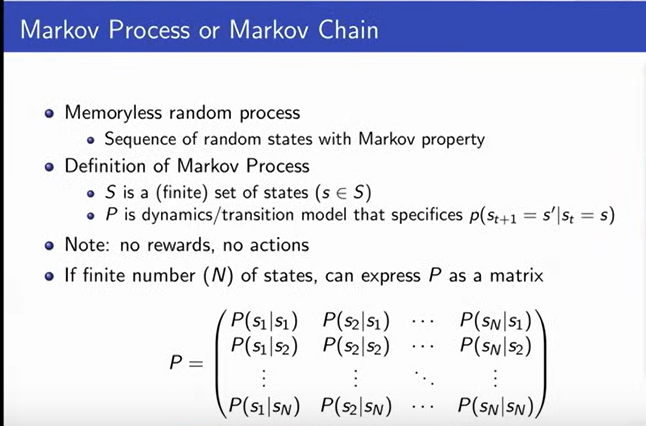
Markov Process or Markov Chain

When we think of a Markov Process or Markov chain, we don't think of a control yet. We don't think of any action. There is no action. But the idea is there will be a scochastic process that's evolving over time.

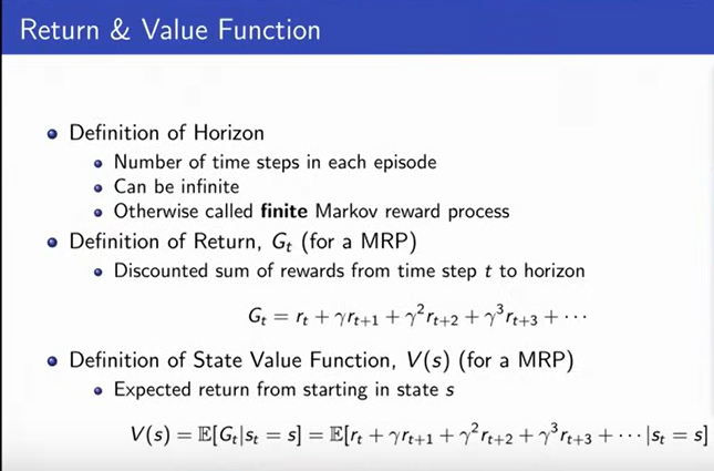
Return & Value Function

When we think about returns, we think about returns and expected returns. We define horizon as how long the agent is acting for. How long this process is going on for and can be infinite. The definition of Return is the sum of rewards from time step. The time can be infinite. Value function is the expected return. If the process is deterministic these two things will be identical. If the process is stochastic, they will be different. That's because in deterministic you always go to same next state. Whereas, it will br different in stochastic process (in general).

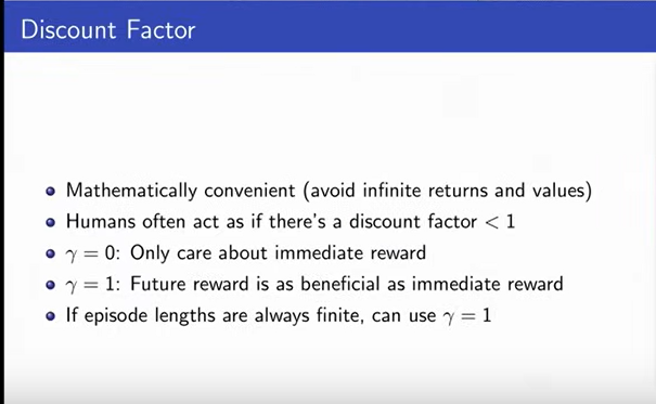
Discount factor

Discount factor- Used for mathematic convenience. We can be assured that the value function is bounded as long as the reward function is bounded. People empirically often act as there is a discount factor. We weigh future rewards lowen than immediate rewards typically. If you are only using discount factor for mathematical convenience, if your horizon is always guaranteed to be finite, its fine to use y (gamma) = 1

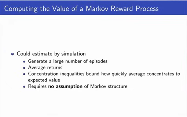
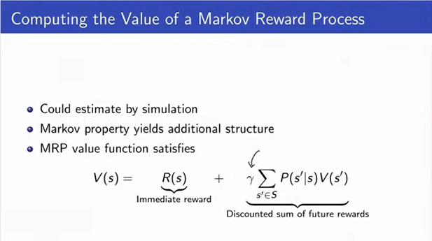
Computing the Value of Markov Reward Process

	The accuracy is given by 1 by square root of n. Where n is the number of roll-outs (simulations). It does not require the process to be markov process. Its just a way to estimate sums of returns. Sums of rewards. It can give you better estimates of process. Which means computationally cheaper ways of estimating what the value of a process.
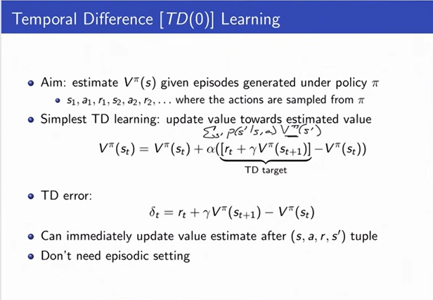
	This means the MRP values is the sum of Immediate reward plus the discounted sum of future rewards.
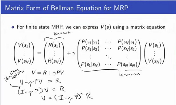
	The figure shows the equation to get V or V(s)
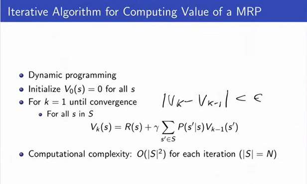
	The computational complexity is lower than the previous method.

Markov Decision Process

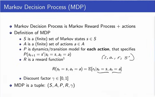
MRP(Markov Reward Process) + action MDP is a tuple which as state, action, reward, dynamics model and discount factor

MDP Policies

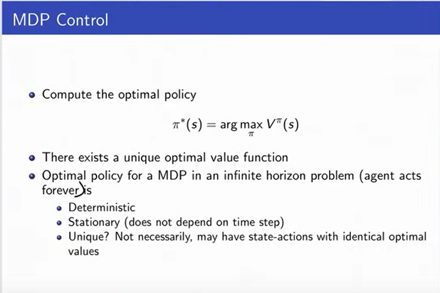
MDP Control

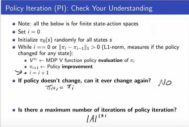
In general if there are |a| actions and |s| states, how many deterministic policies are there? --There are |a| ^ |s| (a to the power s) deterministic policies. Is the optimal policy for a MDP always unique? --NO But there is always an optimal policy which gives maximum return.

Policy Search

If there is unlimited compute power, examine each and every policy and then take the max (reward) of those. But, thats not the case.

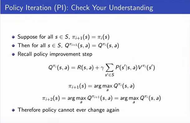
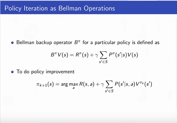
MDP Policy Iteration (PI)

In practice, we keep track of a guess of what the optimal policy might be. We evaluate its value and then we try to improve it. If we can't improve it anymore then we halt. So, we start by initializing randomly. Here now you can think of the subscript is indexing which policy we're at. So, initially we start off with some random policy and then Pi_i is always going to index our current guess of what the optimal policy might be. And while its not changing, we'll talk about whether or not it can change or go back to the same one in a second, we do value function policy. We evaluate the policy using the same sorts of techniques we just discussed because it's a fixed policy. Which means we are now in a markov reward process. And then we do policy improvement. So, the new thing we are doing before now is policy improvement.

New Definition: State-Action Value Q

In order to define how we can improve a policy, we are going to find something new which is the state action value. State values are denoted by V. Which is V_Pi(S) (V Pi of s). Which says if we start in state s and you follow policy pi, what is expected discounted sum of rewards. A state action value says, I will follow this policy pi but not right away. I will take an action a, which might be different than what my policy is telling me to do and then later on the next time-step I'm going to follow policy pi. So, it just says I'm going to get my immediate reward from taking this action a that I am chosing and then I'm going to transition to a new state. Again. that depends on my current state and the action I just took and from then on I am going to take policy pi. So, that defines the Q function.

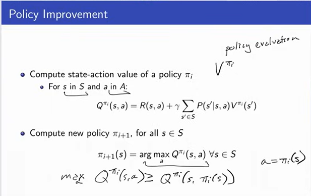
Policy Improvement

What policy improvement does is it takes into consideration a policy, and gets value of it. So, policy evaluation just allowed you to compute what was the value of that policy. And now I want to see if I can improve it. Now, remember right now we are in the case where we know the dynamics model and we know the reward model. So, we proceed with Q computation where we compare the previous value function by policy and now compute Q_pi which is obtained by taking a different action. It could be the same and we do this for all A and for all S. So, for all A and all S we compute this and then we are going to compute the new policy and this is the improvement step which maximizes this Q. So, we do this computation and then we take the max. Now, by definition this has to be greater than or equal to Q_pi(S, pi_(a)) Finding local maxima or global maxima? --Global

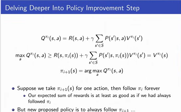
Delving Deeper Into Policy Improvement Step

	First Q function, is calculated. Then new policy is evaluated. For acceptance of new policy, the new value has to be greater than the old value. When we do this, we compute Q function. First we take an action and then we follow our old policy from then onwards. And then I am picking whatever action is maximizing that quantify for each state. Okay. So, I am gonna do this process for each state. But, then we are not going to follow the old policy from that point onwards, we will follow the new policy for all the time. If the new is better.
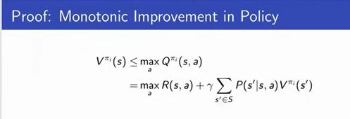
	The value is monotonic if the value of new policy is greater than or equal to the old policy for all states. So, it has to be either the same value or better. With strict inequality if the old policy was suboptimal.

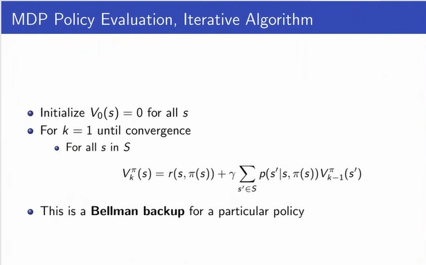
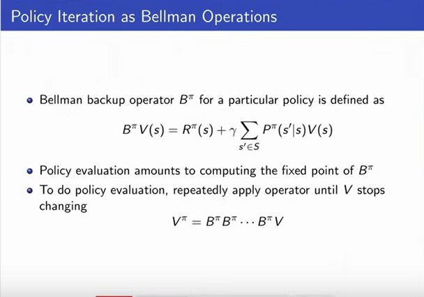
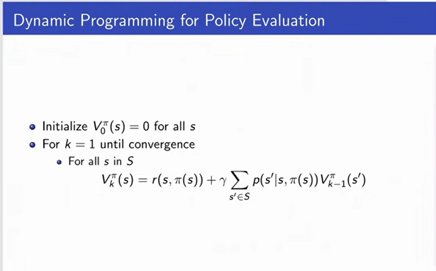
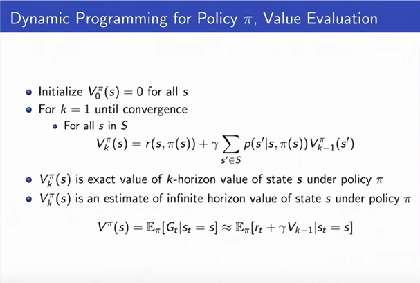
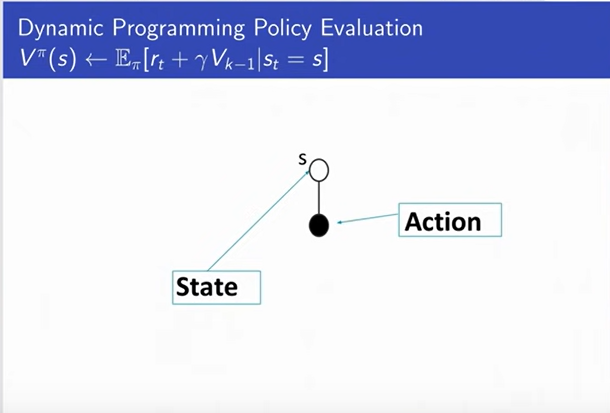
Dynamic Programming for Policy Evaluation

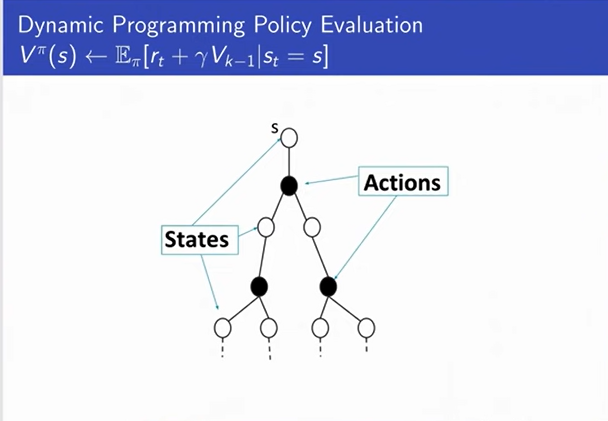
	You are in a state s (denoted with white circle at the top), and then you can take an action. So, what dynamic programming is doing is computing an estimate of the V_pi here at the top by saying, what is the expectation over Pi of RT plus Gamma V_k-1. And that expectation over will be the probalility of s prime given s or P(s'| s1 Pi(s) ). We start with a state and then we take an action, and then we think about the next states that we could reach. We are assuming that we are in a stochastic process. So, we will be at different next state each time. And then we can think about after we reach that state, we can take some other actions. So we can think of drawing the tree of trajectories that we might reach if we started in a state and start following our policy. 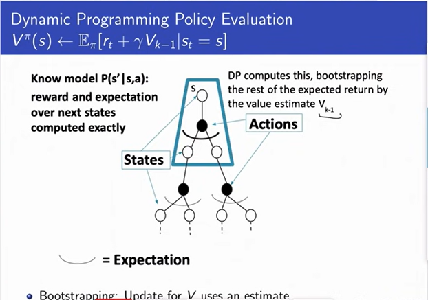Where whenever we get to make a choice, there is a single action we take because we are doing policy evaluation. In dynamic programming we take an expectation over next states.

Policy Evaluation

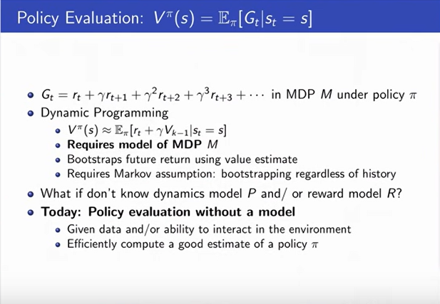
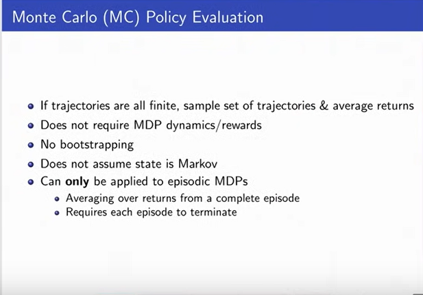
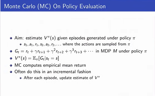
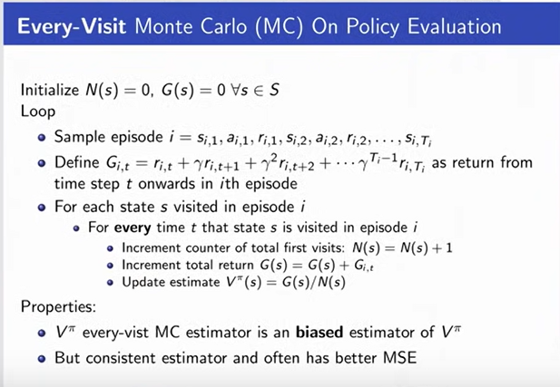
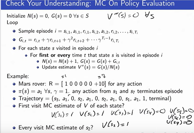
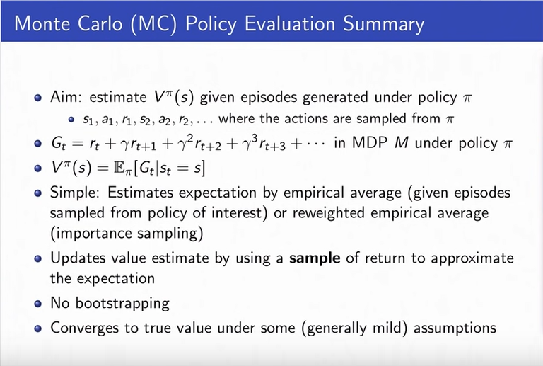
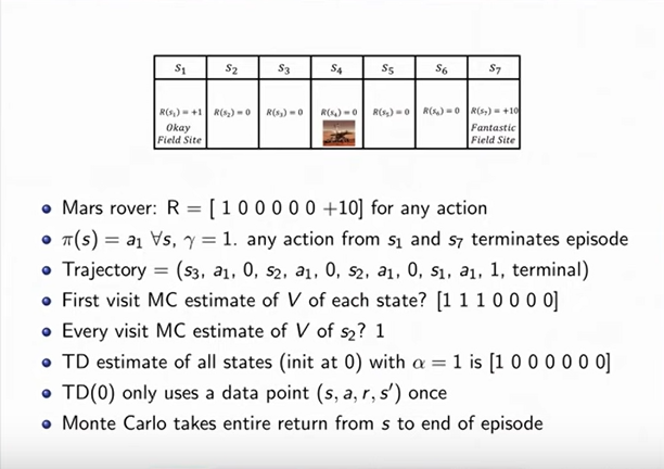
Monte Carlo (MC) Policy Evaluation

• Monte Carlo policy evaluation does not require a specific model of the dynamics/rewards.
• It just requires you to be able to sample from the environment.
• Does not do the bootstraping.
• Does not try to maintian V_k-1.
• It simply sums up all the rewards from each of your trajectories and then averages across those.
• It does not assume that the state is markov.
• There is no notion of the next state and whether or not that summarize the future returns.
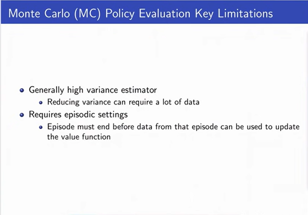
• An important thing is that it can only be applied to episodic MDPs. (The process will end each time.)
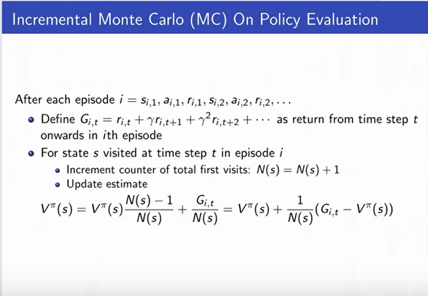
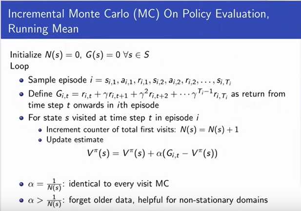
• We also do this in an incremental fashion, which means that after we maintain a runnning estimate, after each episode, we update our current estimate as V_pi. And we hope that as we get more and more data, this estimate will converge to the true value.
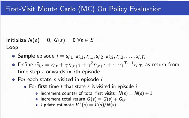
• In the First-Visit slide, N(s) is the number of times visited a state. And then we loop for every timestep t. Increment the counter and update total return. Use average to compute the current estimate of the value for the state. This means consistent (converges to a value).

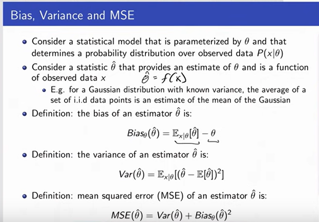
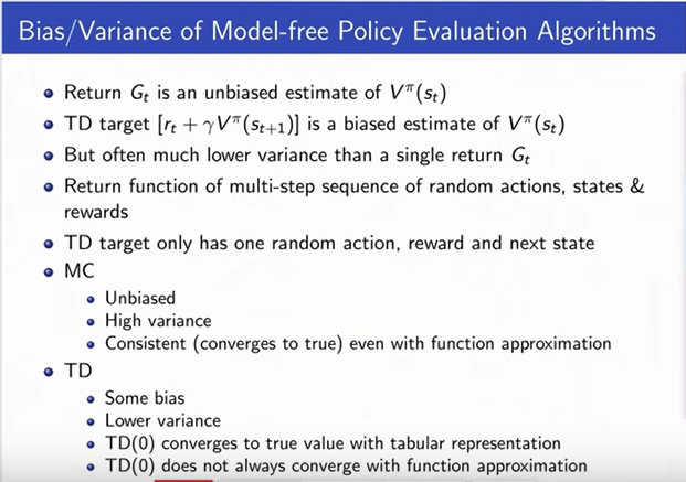
Bias, Variance and MSE

How do we evaluate whether or not the estimate is good? How are we going to compare all of the estimators?

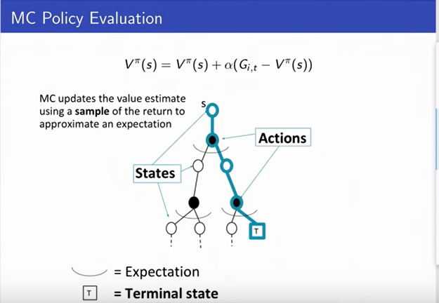
Incremental Monte Carlo On Policy Evaluation

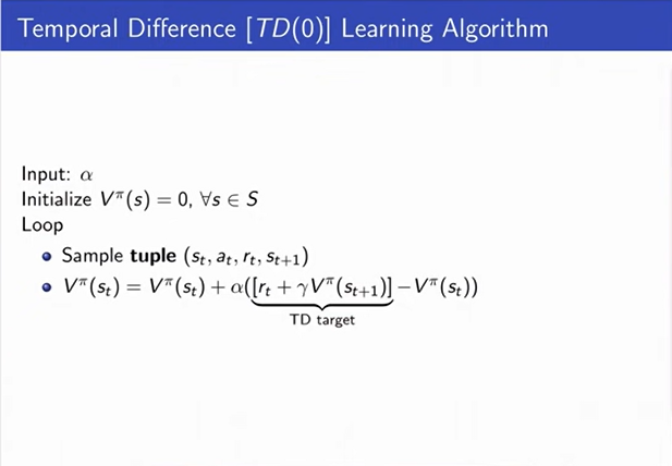
Temporal Difference Learning

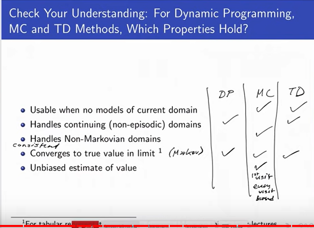
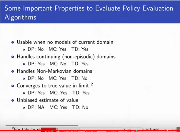
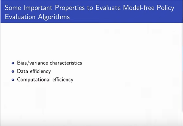
Some Important Properties to evaluate Model-free Policy Evaluation Algorithms

	The differences between MC and TD for mars rover example

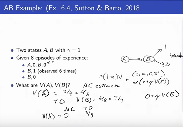
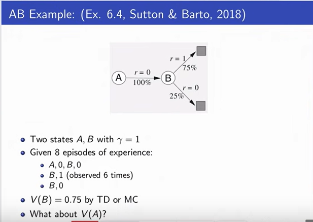
Batch MS and TD

	What if we want to go over data more than once. If they were willing to spend a bit more computation. So we can actually get better estimates and be more sample efficient. Meaning that we want to use our data more effciently so that we can get a better estimate. So often we call this batch or offline. Let's imagine we have set of K episodes, and we can repeatedly smaple an episode. And then we either apply Monte Carlo or TD to the whole episode.

References:

Course content: https://www.youtube.com/playlist?list=PLoROMvodv4rOSOPzutgyCTapiGlY2Nd8u

Content- Stanford CS234: Reinforcement Learning | Winter 2019 | Lecture 1 - Introduction - Emma Brunskill - https://www.youtube.com/watch?v=FgzM3zpZ55o

Content- Stanford CS234: Reinforcement Learning | Winter 2019 | Lecture 2 - Given a Model of the World - https://www.youtube.com/watch?v=E3f2Camj0Is&t=1560s

Content- Stanford CS234: Reinforcement Learning | Winter 2019 | Lecture 3 - Model-Free Policy Evaluation - https://www.youtube.com/watch?v=dRIhrn8cc9w&t=78s

Imitation learning: https://deepai.org/machine-learning-glossary-and-terms/imitation-learning

Menaing of Montezuma's revenge: https://healthcenter.indiana.edu/health-answers/travel/travelers-diarrhea.html